Many thanks to John AC6SL and to Sam WB6RJH for their engaging and well-prepared Tech Talk on ARRL Frequency Measurement Tests (Club Meeting, August 7, 2020). Who knew that wielding electronic instruments and measuring an unmodulated broadcast signal’s frequency would be so interesting! [I did, but I’m a nerd. —Editor.] The aim of the contest is to measure the carrier frequency of an RF signal that is broacast from K5CM in Muskogee OK.

While both John and Sam used the same fundamental method (that is, to measure a frequency accurately, first generate a frequency accurately and then compare) their implementations were different.
John AC6SL
John’s setup (documented in his slides) compares the received signal and a locally generated signal using a Lissajous curve on an oscilloscope. His setup relies on an Electraft K3 Transceiver with a KRX3 High Performance Sub Receiver. In this configuration, both the main and sub receivers are driven by the same local oscillator, meaning that any absolute frequency errors in the receivers cancel. The result is a steady ellipse on the screen of the oscilloscope when the locally generated signal is exactly synchronized with the received signal. Then John uses the frequency of the locally generated signal as the measurement of the received signal’s frequency.
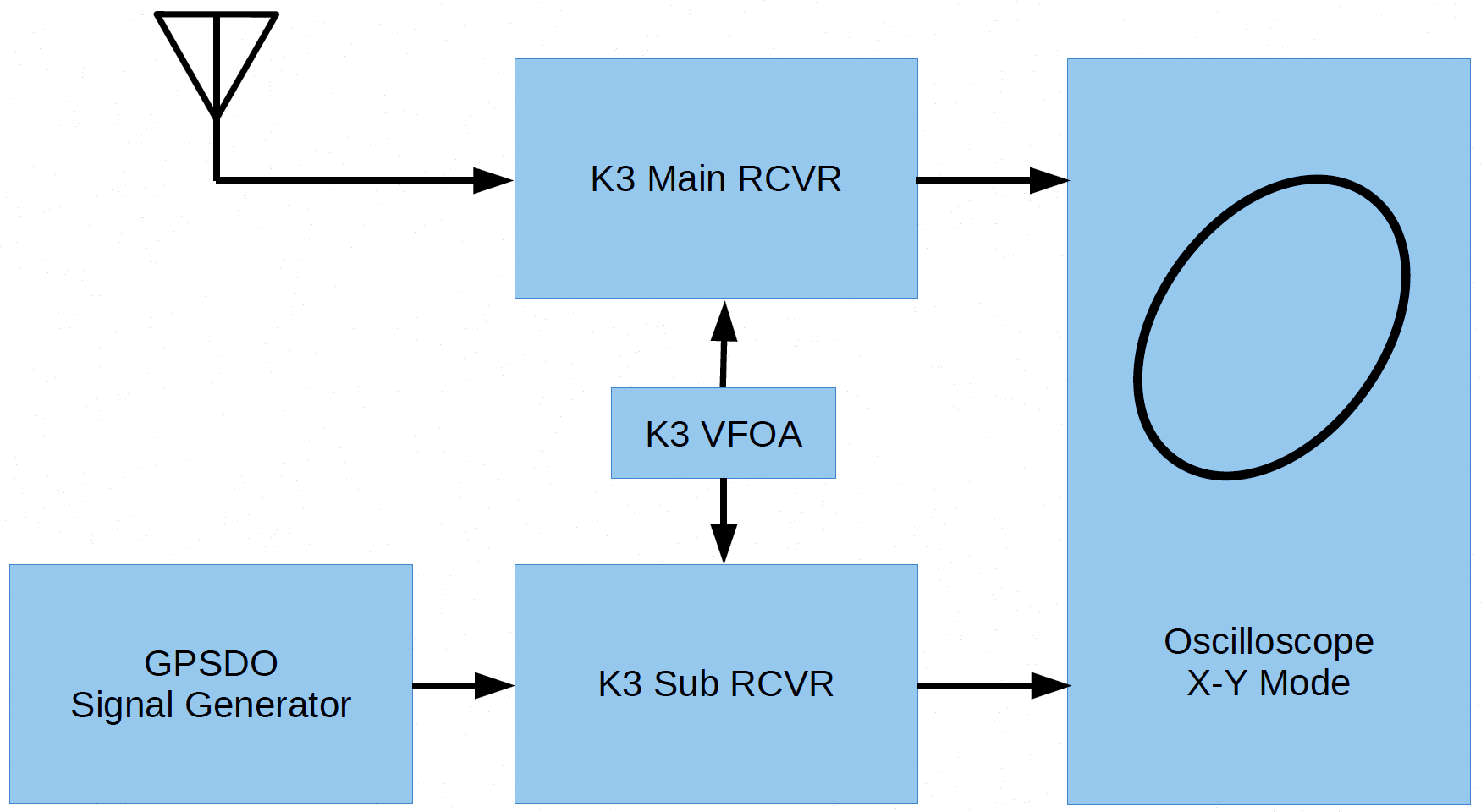
To display the Lissajous curve, John tried using an old Tektronix analog oscilloscope. While it showed a proper curve, the classic instrument was too large for his radio shack, and so he switched to a Linux computer program called xoscope, which displays signals that are sampled from a USB soundcard. It took some finagling to get the software to display an XY curve because the most recent version of the program is missing the XY feature, but John was successful by creating a custom configuration that uses dual trace to emulate an XY display.
In the results, John measured two of the contest’s three transmissions with error less than 1 Hz, but the third measurement was off by much more than expected.
John observes that one disadvantage of his current setup is that rapid tuning is difficult, and so for a future contest he is considering adding a form of computer control.
Sam WB6RJH
While Sam’s overall strategy is the same as John’s (compare a signal of known frequency to a received signal), his implementation is different. (For demonstration and to illustrate ionospheric Doppler shift and turbulence, Sam used WWV at 5 MHz instead of the K5CM FMT signal.) In Sam’s approach, the computer program fldigi is used along with his RF receiver to measure the frequency of the broadcast signal. For comparison, the program also measures the frequency of his highly accurate signal generator, which is set to broadcast about 150 Hz above the K5CM frequency. In this way, as with John’s approach, any errors in the two frequency measurements cancel.
Sam has tuned his measurement instruments to sub-millihertz accuracy, but he observes with irony that his instruments’ capabilities exceed the “accuracy” of the RF path between K5CM and his receiver. As the K5CM signal bounces off of the changing ionosphere, it’s length and phase, and hence, its observed frequency, changes. Sam revealed that changes in the ionosphere cause deviations in the received frequency of up to half a Hz—far exceeding the accuracy of his measurement instruments. And so while Sam has solved the problem of measuring frequency, he now is confronted with the problem of sensing changes in the ionosphere!
While such a feat seems beyond the capabilities of normal humans, during the contest Sam was able to devine the transmitted signals’ actual frequencies from the received signals’ chaotic characteristics and obtain errors of 20 millihertz and 30 millihertz, placing him well inside the top 100-millihertz bracket (do a text search for WB6RJH).
[Thanks to Sam WB6RJH for his technical edits.]